Many calibration technicians follow long-established procedures at their facility that have not evolved with instrumentation technology. Years ago, maintaining a performance specification of ±1% of span was difficult, but today’s instrumentation can easily exceed that level on an annual basis. In some instances, technicians are using old test equipment that does not meet new technology specifications. This article focuses on establishing base line performance testing where analysis of calibration parameters (mainly tolerances, intervals and test point schemes) can be analyzed and adjusted to meet optimal performance. Risk considerations will also be discussed – regulatory, safety, quality, efficiency, downtime and other critical parameters. A good understanding of these variables will help in making the best decisions on how to calibrate plant process instrumentation and how to improve outdated practices.

Introduction

A short introduction to the topics discussed in this post: 

How often to calibrate?

The most basic question facing plant calibration professionals is how often should a process instrument be calibrated? There is not a simple answer, as there are many variables that effect instrument performance and thereby the proper calibration interval, these include:

• Manufacturer’s guidelines (a good place to start)
• Manufacturer’s accuracy specifications
• Stability specification (short term vs. long term)
• Process accuracy requirements
• Typical ambient conditions (harsh vs. climate controlled)
• Regulatory or quality standards requirements
• Costs associated with a failed condition 

Pass/Fail tolerance

The next question for a good calibration program is what is the “Pass/Fail” tolerance? Again, there is no simple answer and opinions vary widely with little regard for what is truly needed to operate a facility safely while producing a quality product at the best efficiency. A criticality analysis of the instrument would be a good place to start. However, tolerance is intimately related to the first question of calibration frequency. A “tight” tolerance may require more frequent testing with a very accurate test standard, while a less critical measurement that uses a very accurate instrument may not require calibration for several years. 

Calibration procedures

What is the best way to determine and implement proper calibration procedures and practices is another question to be answered. In most cases, methods at a particular site have not evolved over time. Many times, calibration technicians follow practices that were set up many years ago and it is not uncommon to hear, “this is the way we have always done it.” Meanwhile, measurement technology continues to improve and is becoming more accurate. It is also getting more complex – why test a fieldbus transmitter with the same approach as a pneumatic transmitter? Performing the standard five-point, up-down test with an error of less than 1% or 2% of span does not always apply to today’s more sophisticated applications. As measurement technology improves, so should the practices and procedures of the calibration technician. 

Finding the optimum...

Finally, plant management needs to understand the tighter the tolerance, the more it will cost to make an accurate measurement. It is a fact that all instruments drift to some degree. It should also be noted that every make/model instrument has a unique “personality” for performance in a specific process application. The only true way to determine optimum calibration parameters is to somehow record calibration in a method that allows performance and drift to be analyzed. With good data and test equipment, the lowest, practical tolerance can be maintained while balancing that with an optimum schedule. Once these parameters are established, associated costs to perform a calibration can be estimated to see if there is justification to purchase a more sophisticated instrument with better performance specifications or purchase more accurate test equipment in order to achieve even better process performance.

Download this article as a free pdf file by clicking the picture below:

Calibration basics 

Optimum calibration interval

Determining a proper calibration interval is an educated guess based on several factors. A best practice is to set a conservative interval based on what the impact of a failure would be in terms of operating in a safe manner while producing product at the highest efficiency and quality. It is also important to review calibration methods and determine the best practices where there will be a minimal impact on plant operations. By focusing on the most critical instruments first, an optimum schedule can be determined and would allow for less critical testing if personnel have availability.

Since all instrumentation drifts no matter the make/model/technology, suppliers end up creating vastly different specifications making it difficult to compare performance. Many times there are several complicating footnotes written in less than coherent terminology. Instrument performance is not always driven by price. The only true way to determine an optimum interval is to collect data and evaluate drift for a specific make/model instrument over time.

Starting off with a conservative interval, after 3 tests, a clear drift pattern may appear. For example, a particular RTD transmitter is tested every three months. The second test indicates a maximum error drift of +0.065 % of span. The third test indicates another +0.060 % of span (+0.125% of span over 6 months). While more data should be used for analysis, a good guess is that this instrument drifts +0.25% per year. Statistically, more data equates to a higher confidence level. If this pattern is common among many of the same make/model RTD transmitters in use throughout the plant, the optimum calibration interval for ±0.50% of span tolerance could be set between 18 to 24 months with a very a relatively high level of confidence.

When collecting data on calibration, it is a good practice to not make unnecessary adjustments. For example, if the tolerance is ±1% of span and the instrument is only out by -0.25% of span, an adjustment should not be made. How can drift be analyzed (minimum of 3 points) with constant adjustment? For certain “personalities,” not adjusting can be a challenge (people strive for perfection), but note that every time an adjustment is made, drift analysis gets more difficult. In general, a best practice is to avoid adjusting until the error is significant. With a consistent schedule, a trim most likely will be needed on the next calibration cycle and not cause an As Found “Fail” condition. Of course, this may not be possible due to criticality, drift history, erratic scheduling or other factors, but when possible, do not automatically make calibration adjustments. 

What if the drift is inconsistent, both increasing, then decreasing over time? More analysis is required; for instance, are the ambient conditions extreme or constantly changing? Depending on the process application, instrument performance may be affected by media, installation, throughput, turbulence or other variables. This situation indicates there is a level of “noise” associated with drift. When this is the case, analysis should show there is a combination random error and systematic error. Random error consists of uncontrollable issues (ambient conditions and process application) vs. systematic error that consists of identifiable issues (instrument drift). By focusing on systematic error and/or clear patterns of drift, a proper calibration interval can be set to maximize operation efficiencies in the safest manner possible.

For more details, there is a dedicated blog post here: How often should instruments be calibrated? 

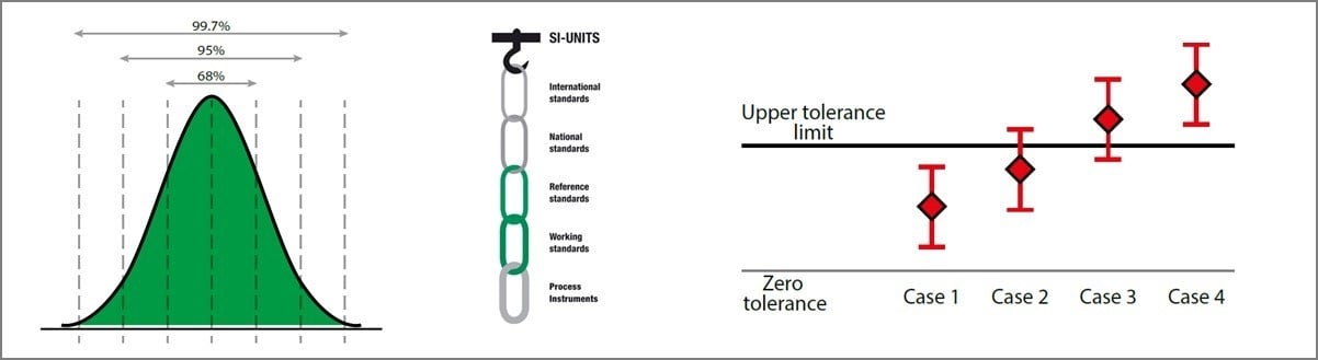
Setting the proper process tolerance limits 

Accuracy, Process Tolerance, Reject Error, Error Limit, Maximum Permissible Error, Error Allowed, Deviation, etc. – these are a few of the many terms used to specify instrument performance in a given process. Transmitter manufacturers always specify accuracy along with several more parameters associated with error (long term stability, repeatability, hysteresis, reference standard and more). When looking at setting a process tolerance, manufacturer accuracy offers a starting point, but it is not always a reliable number. Also, no measurement is better than the calibration standard used to check an instrument. What is behind a manufacturer’s accuracy statement in making an accurate instrument? For pressure, a good deadweight tester in a laboratory should be part of the formula.

At the plant level, a well-known simplified traditional rule of thumb is to have a 4:1 ratio for the calibrator’s uncertainty (total error) vs. the process instrument tolerance (TAR / TUR ratio).

Instead of using the simplified TAR/TUR ratio, the more contemporary approach is to always calculate the total uncertainty of the calibration process. This includes all the components adding uncertainty to the calibration, not only the reference standard.

To learn more on the calibration uncertainty, please read the blog post Calibration Uncertainty for Dummies.

When setting a process tolerance, a best practice is to ask the control engineer what process performance tolerance is required to make the best product in the safest way? Keep in mind the lower the number, the more expensive the calibration costs may be. To meet a tight tolerance, good (more expensive) calibration standards will be required. Also, another issue is to determine whether calibration should be performed in the field or in the shop. If instrumentation is drifting, a more frequent interval will need to be set to catch a measurement error. This may mean increased downtime along with the costs associated with making the actual calibration tests. As an example, review the three graphs of instrument performance:

Example 1 - Tolerance 0.1% of span:

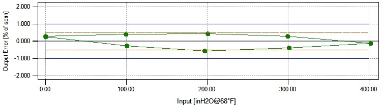
Example 2 - Tolerance 0.25 % of span:

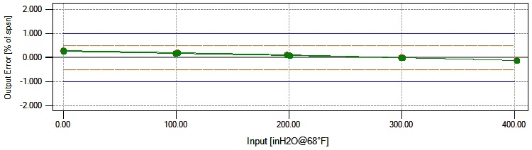
Example 3 - Tolerance 1 % of span:

Note the first graph above shows a failure (nearly double the allowed value), the second shows an adjustment is required (barely passing) and the third shows a transmitter in relative good control. The test data is identical for all 3 graphs, the only difference is the tolerance. Setting a very tight tolerance of ±0.1% of span can cause several problems: dealing with failure reports, constant adjustment adds stress to the calibration technician, operations does not trust the measurement, and more. Graph #2 is not much better, there is not a failure but 0.25% of span is still a tight tolerance and constant adjusting will not allow analysis of drift nor for evaluation of random error or systematic error. There are many benefits in #3 (note that ±1% of span is still a tight tolerance). If a failure were to occur, that would be an unusual (and likely a serious) issue. The calibration technician will spend less time disturbing the process and overall calibration time is faster since there is less adjusting. Good test equipment is available at a reasonable cost that can meet a ±1% of span performance specification.

There may be critical measurements that require a demanding tolerance and thereby accrue higher costs to support, but good judgements can be made by considering true performance requirements vs. associated costs. Simply choosing an arbitrary number that is unreasonably tight can cause more problems than necessary and can increase the stress level beyond control. The best approach would be to set as high a tolerance as possible, collect some performance data and then decrease the tolerance based on a proper interval to achieve optimum results. 

Calibration parameters

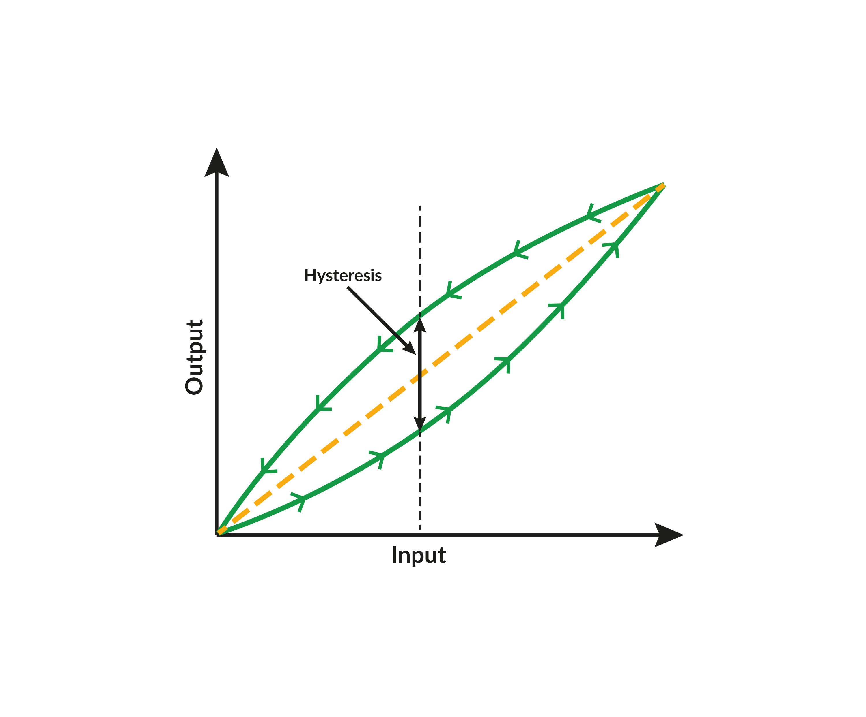
A subtle yet important detail is to review calibration procedures to see if further efficiencies can be gained without impacting the quality of the data. Years ago, technology was more mechanical in nature, board components were more numerous/complex, and instruments were more sensitive to ambient conditions. Today’s smart technology offers better accuracy and “brain power” with less, simplified components and with improved compensation capabilities. In many cases, old testing habits have not evolved with the technology. A good example is an older strain gauge pressure sensor that when starting from zero “skews” toward the low side as pressure rises due to the change from a relaxed state. Likewise, when the sensing element is deflected to its maximum pressure and as the pressure then decreases, there is a mechanical memory that “skews” the measure pressure toward the high end. This phenomenon is called hysteresis and graphically would resemble the graph below when performing a calibration:

5-point Up/Down calibration with hysteresis:

Today’s smart pressure sensors are much improved, and hysteresis would only occur if something were wrong with the sensor and/or it is dirty or has been damaged. If the same calibration was performed on a modern sensor, the typical graphical representation would look like this:

5-point Up/Down calibration with no hysteresis:

This may look simple, but it takes significant effort for a calibration technician to perform a manual pressure calibration with a hand pump. Testing at zero is easy, but the typical practice is to spend the effort to hit an exact pressure test point in order to make an error estimate based on the “odd” mA signal. For example, if 25 inH₂O is supposed to be exactly 8 mA, but 8.1623 mA is observed when the pressure is set to exactly 25 inH₂O, an experienced technician knows he is dealing with a 1% of span error (0.1623 ÷ 16 x 100 = 1%). This extra effort to hit a “cardinal” test point can be time consuming, especially at a very low pressure of 25 in H₂O. To perform a 9-point calibration, it might take 5 minutes or more and makes this example calibration unnecessarily longer. It is possible to perform a 5-point calibration and cut the time in half – the graph would look identical as the downward test points are not adding any new information. However, a pressure sensor is still mechanical in nature and, as mentioned, could have hysteresis. on a pressure transmitter. The quality of the test point data is equivalent to a 9-point calibration and if there is hysteresis, it will be detected. This also places the least stress on the technician as there are only 3 “difficult” test points (zero is easy) compared to 4 points for a 5-point calibration and 7 for a 9-point up/down calibration. Savings can be significant over time and will make the technician’s day to day work much easier.

Using this same approach can work for temperature instrumentation as well. A temperature sensor (RTD or thermocouple) is electromechanical in nature and typically does not exhibit hysteresis – whatever happens going up in temperature is repeatable when the temperature is going down. The most common phenomenon is a “zero shift” that is indicative of a thermal shock or physical damage (rough contact in the process or dropped). A temperature transmitter is an electronic device and with modern smart technology exhibits excellent measurement properties. Therefore, a best practice is to perform a simple 3-point calibration on temperature instrumentation. If calibrating a sensor in a dry block or bath, testing more than 3 points is a waste of time unless there is a high accuracy requirement or some other practical reason to calibrate with more points.

There are other examples of optimizing parameters. Calibration should relate to the process; if the process never goes below 100°C, why test at zero? When using a dry block, it can take a very long time to reach a test point of 0°C or below – why not set an initial test point of 5°C with an expected output of 4.8 mA, for example, if it is practical and will save time and make calibrating easier. Another good example is calibrating a differential pressure flow meter with square root extraction. Since a flow rate is being measured, output test points should be 8 mA, 12 mA, 16 mA and 20 mA, not based on even pressure input steps. Also, this technology employs a “low flow cut-off” where very low flow is not measurable. A best practice is to calibrate at an initial test point of 5.6 mA output (which is very close to zero at just 1% of the input span).

Do not overlook how specific calibrations are performed. Why collect unnecessary data? It is simply more information to process and can have a very significant cost. Why make the job of calibration harder? Look at the historical data and make decisions that will simplify work without sacrificing quality.

Calibration trend analysis and cost 

Temperature transmitter example

 As mentioned, the best way to optimize calibration scheduling is to analyze historical data. There is a balance of process performance vs. instrument drift vs. tolerance vs. optimum interval vs. cost of calibration and the only way to truly determine this is through historical data review. Using similar data for the temperature transmitter example in the Tolerance Error Limits section, apply the concepts to optimize the calibration schedule with this scenario:  

Calibration history trend example:

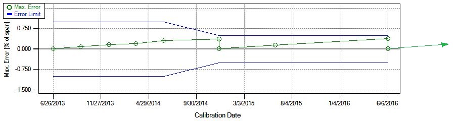
After a discussion between the Control Engineer and the I&C Maintenance group, a case was made for a tolerance of ±0.5% of span, but it was agreed that ±1% of span was acceptable until more information becomes available. This particular measurement is critical, so it was also agreed to calibrate every 3 months until more information becomes available. At the end of the first year, a drift of approximately +0.25% of span per year was observed and no adjustments were made. After further discussion, it was agreed to lower the tolerance to ±0.5% of span (the Control Engineer is happy) and to increase the interval to 6 months. An adjustment was finally made 1-1/2 years after the initial calibration. At the end of year 2, no adjustment was required and the interval was increased to 1 year. At the end of year 3, an adjustment was made, and the interval was increased to 18 months (now the Plant Manager, the I&C Supervisor and the I&C Technicians are happy). All this occurred without a single failure that might have required special reporting or other headaches.

Obviously this scenario is perfect, but if there are multiple instruments of the same make/model, strong trends will emerge with good historical data; affirming best practices and allowing best decisions to be made. For critical instrument measurements, most engineers are conservative and “over-calibrate”.  This example should open a discussion on how to work smarter, save time/energy and maintain a safe environment without compromising quality.

Cost of calibration

One other best practice is whenever possible, try to establish the cost to perform a given calibration and include this in the decision process. Consider not only the man hours, but the cost of calibration equipment, including annual recertification costs. When discussing intervals and tolerances, this can be very important information in making a smart decision. Good measurements cannot be made with marginal calibration equipment. As an example, in order to meet an especially tight pressure measurement tolerance, a deadweight tester should be used instead of a standard pressure calibrator – this is a huge step in equipment cost and technician experience/training. By outlining all the extra costs associated with such a measurement, a good compromise could be reached by determining the rewards vs. risks of performing more frequent calibrations with slightly less accurate equipment or by utilizing alternative calibration equipment.

Another overlooked operational cost is the critical need to invest in personnel and equipment. With either new technology or new calibration equipment, maintenance and/or calibration procedures should be reinforced with good training. ISA offers several excellent training options and consider local programs that are available for calibration technicians via trade schools or industry seminars. Finally, a review of calibration assets should be done annually to justify reinvestment by replacing old equipment. Annual recertification can be expensive, so when choosing new calibration equipment, look for one device that can possibly replace multiple items.

One other important cost to consider is the cost of failure. What happens when a critical instrument fails? If there are audits or potential shut-down issues, it is imperative to have a good calibration program and catch issues before they begin in order to avoid a lengthy recovery process. If calibration equipment comes back with a failed module, what is the potential impact on all the calibrations performed by that module in the past year? By understanding these risks and associated costs, proper decisions and investments can be made.

Conclusion

Obviously, not all instrumentation is going to offer easy analysis to predict drift. Also, calibration schedules get interrupted and many times work has to be done during an outage regardless of careful planning. In some areas there are regulatory requirements, standards or quality systems that specify how often instrument should be calibrated – it is difficult to argue with auditors. A best practice is to establish a good program, focusing on the most critical instruments. As the critical instruments get under control, time will become available to expand to the next level of criticality, and on and on.

Alternate or “hybrid” strategies should be employed in a good calibration management program. For example, loop calibration can lower calibration costs, which is performing end-to-end calibrations and only checking individual instruments when the loop is out. A good “hybrid” strategy is to perform a “light” calibration schedule combined with a less frequent “in-depth” calibration. As an example, make a minimally invasive “spot check” (typically one point) that has a lower tolerance than normal (use the recommended 2/3 of the normal tolerance value). Should the “spot check” fail, the standard procedure would be to perform the standard in-depth calibration to make necessary adjustments. A technician may have a route of 10 “spot checks” and end up only performing 1 or 2 in-depth calibrations for the entire route. Performing “spot checks” should still be documented and tracked, as good information about drift can come from this type of data.

To summarize, several best practices have been cited:

• Set a conservative calibration interval based on what the impact of a failure would mean in terms of operating in a safe manner while producing product at the highest efficiency and quality.
• Try not to make adjustments until the error significance exceeds 50% (or greater than ±0.5% for a tolerance of ±1% of span); this may be difficult for a technician striving for perfection, however, when unnecessary adjustments are made, drift analysis is compromised.
• Ask the control engineer what process performance tolerance is required to make the best product in the safest way?
• Set as high a tolerance as possible, collect some performance data and then decrease the tolerance based on a proper interval to achieve optimum results.
• Perform a 3-point up/down calibration on a pressure transmitter; the quality of the test point data is equivalent to a 9-point calibration and if there is hysteresis, it will be detected.
• Perform a simple 3-point calibration on temperature instrumentation. If calibrating a sensor in a dry block or bath, calibrating more than 3 points is a waste of time unless there is a high accuracy requirement or some other practical reason to calibrate with more points.
• Calibrate a differential pressure flow transmitter with square-root extraction at an initial test point of 5.6 mA output (which is very close to zero at just 1% of the input span). Also, since a flow rate is being measured, the sequential output test points should be 8 mA, 12 mA, 16 mA and 20 mA, not based on even pressure input steps.
• Whenever possible, try to establish the cost to perform a given calibration and include this in the decision process.
• Focus on the most critical instruments, establish a good program and as the critical instruments get under control, time will become available to expand to the next level of criticality, and on and on.

Always keep in mind that instruments drift, some perform better than others. The performance tolerance set will ultimately determine the calibration schedule. Via documentation, if there will be capability to distinguish systematic error (drift) from random error ("noise") and a systematic pattern emerges, an optimal calibration interval can be determined. The best tolerance/interval combination will provide good control data for the best efficiency, quality and safety at the lowest calibration cost with minimal audit failures and/or headaches. Establishing best practices for calibration should be a continuous evolution. Technology is changing and calibration should evolve along with it. As discussed, there are many variables that go into proper calibration – by establishing base line performance, as observed in the operating environment, smart decisions can be made (and modified) to operate at optimal levels when it comes to calibration.

Download this article as a free pdf file by clicking the picture below:

Beamex CMX Calibration Management software

All graphics in this post have been generated using the Beamex CMX Calibration Management software.

Related blog posts

You might find these blog posts interesting:

• How often should instruments be calibrated?
• Measurement Uncertainty: Calibration uncertainty for dummies - Part 1
• Using Metrology Fundamentals in Calibration to Drive Long-Term Value
• How to avoid common mistakes in field calibration [Webinar] 
• Calibration Out of Tolerance: What does it mean and what to do next? - Part 1 of 2