Calibrating a square rooting pressure transmitter

We quite often receive questions regarding the calibration of a square rooting pressure transmitter.  Most often the concern is that the calibration fails too easily at the zero point. There is a reason for that, so let’s find out what that is.

First, when we talk about a square rooting pressure transmitter, it means a transmitter that does not have a linear transfer function, instead, it has a square rooting transfer function. When the input pressure changes, the output current changes according to a square rooting formula. For example, when the input is 0% the output is 0% of the range, just as when input is 100% output is 100%. But when the input is only 1% the output is already 10%, and when the input is 4% output is 20%. The picture later explains this graphically.

So, why and when would you use that kind of transmitter? It is used when you are measuring flow with a differential pressure transmitter. In case you have some form of restriction structure (orifice/venturi) in your pipe the bigger the flow is, the more pressure is generated over that structure. When the flow grows the pressure does not grow linearly, it grows with a quadratic correlation.

If you want to send a mA signal to your control room, you use a square rooting pressure transmitter that compensates for the quadratic correlation - and as a result, you have a mA signal that is linear to the actual flow signal. You could also use a linear pressure transmitter and make the conversion calculation in your DCS system, ISO-5167 gives more guidance.

So, what about when you start calibrating this kind of square rooting transmitter?

You can, of course, calibrate it in a normal way, by injecting a known pressure to the transmitter’s input and measuring the mA output. You should anyhow remember that the output current does not change linearly when the input pressure changes. Instead, the mA output grows according to the rooting transfer function. This means that in the beginning, when you are at zero input and you have 4 mA output, the transfer function is VERY steep. Even the smallest change in the pressure will cause the output to change a lot. I have illustrated this in the simple figure below. The red curve shows the transfer function of a square rooting transmitter and the blue line shows the function of a linear transmitter.

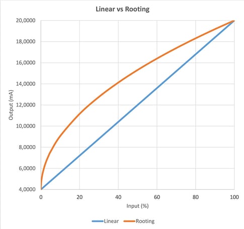
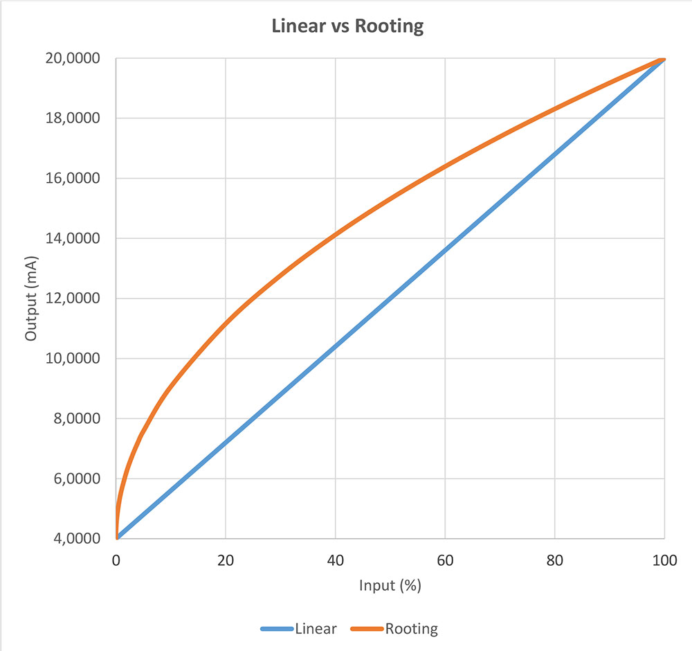Figure 1. Linear versus square rooting.

In practice, this means that if your input pressure measurement fluctuates just one or a few digits, the output should change a lot in order for the error to be zero. What happens is that if the measured values fluctuates even in the least significant digit, the error calculation will say that the point fails. In practice, it is just about impossible to make that zero point to be a “Pass” calibration point within the allowed tolerance.

So what to do? In order to calibrate, you should simply move the first calibration point a bit higher than 0% of the input range. If the first calibration point is at 5 – 10% of the input range, you are already out of the steepest part of the curve and you can get reasonable readings and error calculation. Of course, then you don’t calibrate the zero point, but your process is normally not running at zero point either.

I hope this short explanation made some sense and helped with this issue, let me know if you need any further explanations!

Yours truly,
Heikki

Update, Feb 2018:

How to calculate the output?

There have been some questions on how to calculate the output mA of a square rooting pressure transmitter.

Below is a formula that you can use to calculate what the output current should be at a given input point:

Where:

Heikki Laurila is Product Marketing Manager at Beamex Oy Ab. He started working for Beamex in 1988 and has, during his years at Beamex, worked in production, the service department, the calibration laboratory, as quality manager and as product manager. Heikki has a Bachelor's degree in Science.
Heikkis family consists of himself, his wife and their four children. In his spare time he enjoys playing the guitar.